P3 features
While the pipeline is generic enough to support arbitrary numbers of arbitrary features, here we describe the actual features used. This section can be used as a starting point for creating custom sets of features for other types of data.
Each set of features requires a different set of pre-processing steps. To
accommodate this, and to isolate the customization into discrete,
easily-editable components, features are handled by separate workflows. In some
cases, the workflows are interdependent on each other. Each workflow is expected to
create the output files defined in the config.yaml file.
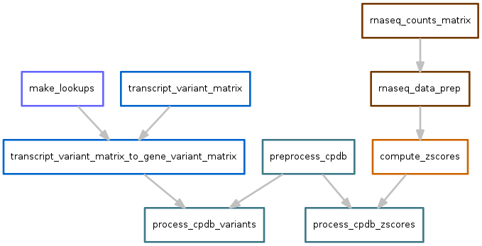
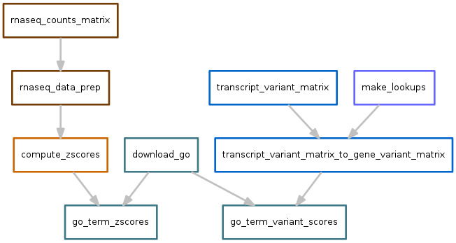
Below, each sub-workflow is shown separately as a directed acyclic graph (DAG) of the tasks performed and the first few lines of the output file (or files) are shown. To illustrate interdepdencies among workflows, sub-workflows have been color coded.
Snakefile

norm_counts.snakefile
This workflow starts with htseq-count files, one for each sample. They have the following format:
GENE_ID	counts
ENSG00000234515	8435
ENSG00000264113	0
ENSG00000243514	0
ENSG00000103415	0
The workflow is the following:
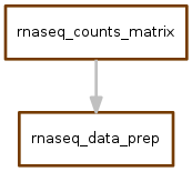
The output file of norm_counts.snakefile is a table of gene-level
quantile-normalized counts per million (CPM). One row per gene, and one column
per sample:
LineA_1	LineB_2	LineC_3	LineD_4	LineE_5	LineF_6	LineG_7	LineH_8	LineI_9	LineJ_10
ENSG00000234515	17.8687589559481	1.0769198527651	-1	-1	4.82703381950925	6.38863928575311	-1	-1	5.68281394137488	-1
ENSG00000264113	-1	-1	-1	17.8687589559481	-0.0576641927637963	-1	12.1996591413175	16.6358805540731	7.30331969731323	17.8687589559481
ENSG00000243514	-1	1.0769198527651	-1	2.50532392304214	-1	14.2884920493533	13.065890821649	-1	15.3885252912467	-1
ENSG00000103415	-1	11.0105207510527	4.32755526660216	12.1996591413175	2.50532392304214	5.24816249855466	11.7813206156511	-1	-1	8.8974528747595
zscores.snakefile
This workflow takes the output of norm_counts.snakefile and converts counts into zscores. In the absence of matched controls, these zscores are then used as a proxy for direction and magnitude of differential expression.
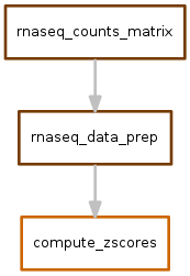
Output looks like this:
LineA_1	LineB_2	LineC_3	LineD_4	LineE_5	LineF_6	LineG_7	LineH_8	LineI_9	LineJ_10
ENSG00000234515	11.580968729376	0.674490759476595	-0.674490759476595	-0.674490759476595	3.11022963903472	4.12450898691359	-0.674490759476595	-0.674490759476595	3.66606792386179	-0.674490759476595
ENSG00000264113	-0.674490759476595	-0.674490759476595	-0.674490759476595	2.07854358239692	-0.53699984950445	-0.674490759476595	1.25139715937969	1.8986612389084	0.53699984950445	2.07854358239692
ENSG00000243514	-0.674490759476595	0.674490759476595	-0.674490759476595	1.60225438494143	-0.674490759476595	9.25554732060764	8.46145482877324	-0.674490759476595	9.97003060294169	-0.674490759476595
ENSG00000103415	-0.674490759476595	0.7251607226062	-0.053641690619681	0.863737504149148	-0.26599624656081	0.053641690619681	0.814986234358453	-0.674490759476595	-0.674490759476595	0.478913399438626
variants.snakefile
Todo
Need more methods here about how the original data files were processed.
The starting point of the exome variant data are tab-delimited files, one for each sample, generated by running SnpEff on VCF files, performing filtering steps to exclude likely germline mutations, and excluding the VCF header:
#CHROM	POS	ID	REF	ALT	1000G	COSMIC	DB	NHLBI	EFF[*].EFFECT	EFF[*].IMPACT	EFF[*].FUNCLASS	EFF[*].CODON	EFF[*].AA	EFF[*].AA_LEN	EFF[*].GENE	EFF[*].BIOTYPE	EFF[*].CODING	EFF[*].TRID	EFF[*].RANK	GEN[0].AD[0]	GEN[0].AD[1]	GEN[0].DP
6	30994026	.	C	C	.	.	.	.	NON_SYNONYMOUS_CODING	MODERATE	MISSENSE	.	.	.	MUC22	protein_coding	CODING	ENST00000561890	.	.	.	.
7	129825046	.	G	T	.	.	.	.	CODON_CHANGE_PLUS_CODON_DELETION	MODERATE	.	.	.	.	TMEM209	protein_coding	CODING	ENST00000397622	.	.	.	.
12	72070805	.	G	C	.	.	.	.	NON_SYNONYMOUS_CODING	MODERATE	MISSENSE	.	.	.	THAP2	protein_coding	CODING	ENST00000308086	.	.	.	.
19	58514095	.	A	TGCC	.	.	.	.	CODON_INSERTION	MODERATE	.	.	.	.	CTD-2368P22.1	protein_coding	CODING	ENST00000550135	.	.	.	.
SnpEff reports effects on a per-transcript basis. For integration with other features that consider genes (i.e., the pathway features), after collecting samples into a transcripts x sample matrix, we aggregate into a gene x sample matrix by summing variants across all transcripts of a gene.
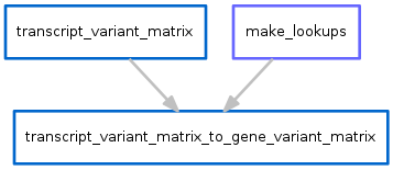
Output of the gene x sample matrix looks like this, where values indicate the total number of variants across a gene in a sample.
Specifically, since the variants in these files have been pre-filtered to only contain those with high impact, the value for each gene represents the total number of rows in the VCF file annotated with transcript IDs (EFF[*].TRID column) belonging to that gene.
ENSEMBL	LineA_1	LineB_2	LineC_3	LineD_4	LineE_5	LineF_6	LineG_7	LineH_8	LineI_9	LineJ_10
ENSG00000005238	0.0	0.0	0.0	1.0	0.0	0.0	0.0	0.0	0.0	0.0
ENSG00000005483	1.0	0.0	0.0	0.0	0.0	0.0	0.0	0.0	0.0	0.0
ENSG00000006377	0.0	0.0	1.0	0.0	0.0	0.0	0.0	0.0	0.0	0.0
ENSG00000006788	0.0	0.0	0.0	0.0	0.0	0.0	0.0	0.0	0.0	1.0
cnv.snakefile
The copy number variation (CNV) data starts as files in SEG format for each sample. For example:
ID	chrom	loc.start	loc.end	num.mark	seg.mean
LineA_1	1	564454	746638	1594	0.0155
LineA_1	1	752741	12846964	1205	0.3181
LineA_1	1	12866220	12912597	8	-0.554
LineA_1	1	12917433	22050665	3	-4.111
Todo
Need methods on how the SEG files were created
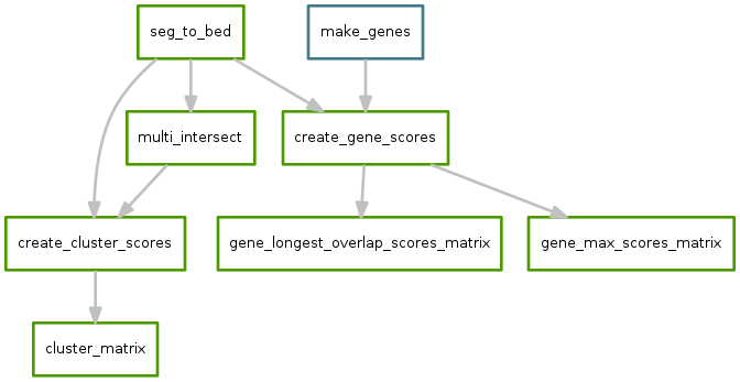
Since each sample may have a different set of CNVs, the total number of unique CNVs across all samples must be determined. The multiinter program from the BEDTools suite is used to identify a uniform set of segments that can be used across all samples.
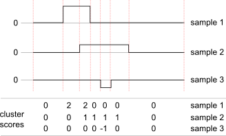
This uniform set of segments is then intersected with the actual segments on a per-sample basis to obtain per-sample CNV values for each segment. Files across samples are then aggregated into a single “cluster matrix” file.
This diagram shows how cluster scores are calculated for a hypothetical set of 3 samples:
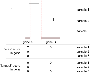
A separate set of scores is calculated at the gene level. A score for each gene can be calculated in several ways. The following diagram shows two ways: the largest magnitude CNV that overlaps the gene (“max”), or the score of the longest segment that overlaps the gene (“longest”):
The final cluster scores output file looks like the following:
cluster_id	LineG_7	LineH_8	LineD_4	LineB_2	LineA_1	LineF_6	LineJ_10	LineI_9	LineE_5	LineC_3
1_746638_752741	-0.9704	0.563	-0.6339	-0.3851	0.0	0.0095	-3.3	-3.252	-1.3537	1.1942
1_752741_1613780	-0.9704	0.563	-0.6339	-0.3851	0.3181	0.0095	-3.3	-3.252	-1.3537	1.1942
1_1613780_1651398	-0.9704	0.563	-0.6339	-0.3851	0.3181	0.0095	-3.3	0.0	-1.3537	1.1942
1_1651398_1664194	-0.9704	0.563	-0.6339	-0.3851	0.3181	0.0095	-3.3	-1.6732	-1.3537	1.1942
And the “max” gene scores:
gene_id	LineH_8	LineE_5	LineI_9	LineB_2	LineC_3	LineF_6	LineG_7	LineA_1	LineJ_10	LineD_4
ENSG00000000003	0.5661	0.6118	0.0424	-0.0806	-1.3841	0.0537	-0.6318	0.8189	0.5658	-1.6282
ENSG00000000005	0.5661	0.6118	0.0424	-0.0806	-1.3841	0.0537	-0.6318	0.8189	0.5658	-1.6282
ENSG00000000419	-1.3006	1.3093	-0.9166	-0.517	0.3748	-1.0073	-4.5621	0.3678	-1.4437	0.2662
ENSG00000000457	-0.2612	-0.5819	-2.4134	0.2732	0.6348	0.5559	-1.4232	-0.9155	-4.2292	-0.5872
And the “longest” gene scores:
gene_id	LineH_8	LineA_1	LineB_2	LineG_7	LineE_5	LineJ_10	LineD_4	LineC_3	LineF_6	LineI_9
ENSG00000000003	0.5661	0.8189	-0.0806	-0.6318	0.6118	0.5658	-1.6282	-1.3841	0.0537	0.0424
ENSG00000000005	0.5661	0.8189	-0.0806	-0.6318	0.6118	0.5658	-1.6282	-1.3841	0.0537	0.0424
ENSG00000000419	-1.3006	0.3678	-0.517	-4.5621	1.3093	-1.4437	0.2662	0.3748	-1.0073	-0.9166
ENSG00000000457	-0.2612	-0.9155	0.2732	-1.4232	-0.5819	-4.2292	-0.5872	0.6348	0.5559	-2.4134
Pathways
Several annotation databases are used. These databases have annotations for each gene in a gene x annotation file. However, the features need to be in a annotation x samples file for use with regression methods. Therefore these pathway workflows use different strategies to calculate a pathway score for each sample, based on some property or properties of the genes for that pathway in that sample.
See Obtaining pathway scores for more details.
In the pathway workflows below, there are several “flavors” of scores, each of which are derived from workflows described above. For example, there are scores derived from zscores, variants, and CNV data.
Consensus pathway database
Scores for each pathway are calculated based on the output of variants.snakefile and zscores.snakefile.
Variants output file:
pathway_id	LineA_1	LineB_2	LineC_3	LineD_4	LineE_5	LineF_6	LineG_7	LineH_8	LineI_9	LineJ_10
N-Glycan_biosynthesis_sum_var	0.0	0.0	1.0	0.0	0.0	0.0	0.0	0.0	0.0	0.0
None_sum_var	0.0	0.0	0.0	0.0	0.0	0.0	0.0	0.0	1.0	0.0
PA152241951_sum_var	0.0	0.0	0.0	0.0	0.0	0.0	0.0	0.0	1.0	0.0
Pathway_EGFR1_sum_var	0.0	1.0	4.0	1.0	1.0	1.0	3.0	1.0	2.0	1.0
Zscores output file:
pathway_id	LineA_1	LineB_2	LineC_3	LineD_4	LineE_5	LineF_6	LineG_7	LineH_8	LineI_9	LineJ_10
N-Glycan_biosynthesis_sum_pos		0.6744907594765949	3.5638961701333796				1.03207331666923	4.1439504657554		3.00806348507059
None_sum_pos	0.131088071579741		1.4664123740802788	0.8307047838158309	0.32206503184169205	2.8771587960372305	1.8697663658591699	1.5811716854272402	0.407459235642265
PA152241951_sum_pos	1.3566355942144999		0.423897601727489		0.157361464312241		1.14508070430709			0.554828755663669
PWY-5874_sum_pos		0.7251607226062		0.8637375041491481		0.053641690619681	0.814986234358453			0.47891339943862604
Gene ontology
Scores for each GO term are calculated based on the output of variants.snakefile and zscores.snakefile.
Variants output file:
pathway_id	LineA_1	LineB_2	LineC_3	LineD_4	LineE_5	LineF_6	LineG_7	LineH_8	LineI_9	LineJ_10
GO_0000122_sum_var	0.0	0.0	0.0	0.0	0.0	0.0	0.0	0.0	1.0	0.0
GO_0000978_sum_var	0.0	0.0	0.0	0.0	0.0	0.0	0.0	0.0	1.0	0.0
GO_0001077_sum_var	0.0	0.0	0.0	0.0	0.0	0.0	0.0	0.0	1.0	0.0
GO_0001133_sum_var	0.0	0.0	0.0	0.0	0.0	0.0	0.0	0.0	1.0	0.0
Zscores output file:
pathway_id	LineA_1	LineB_2	LineC_3	LineD_4	LineE_5	LineF_6	LineG_7	LineH_8	LineI_9	LineJ_10
GO_0000122_sum_pos	2.3518180778796096	1.76273485147185	0.694044921834633	3.9069612972010397	1.4971888921138388	0.9013622016070708	2.694214312746489		2.040518117783778
GO_0000159_sum_pos	2.48468185483921		1.69424387076123		1.1789473338098202	0.8296420036025209			0.597470904863933
GO_0000287_sum_pos	1.3566355942144999		0.423897601727489		0.157361464312241		1.14508070430709			0.554828755663669
GO_0000775_sum_pos	2.48468185483921		1.69424387076123		1.1789473338098202	0.8296420036025209			0.597470904863933
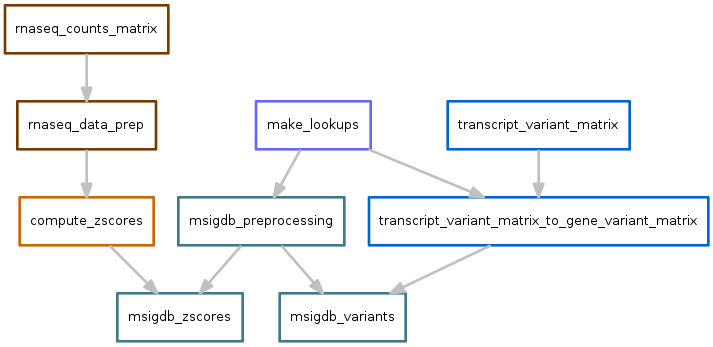
MSIG database
Scores for each pathway are calculated based on the output of variants.snakefile and zscores.snakefile.
Variants output file:
pathway_id	LineA_1	LineB_2	LineC_3	LineD_4	LineE_5	LineF_6	LineG_7	LineH_8	LineI_9	LineJ_10
KEGG_CHEMOKINE_SIGNALING_PATHWAY_sum_var	0.0	0.0	1.0	0.0	1.0	0.0	1.0	0.0	0.0	0.0
KEGG_CYTOKINE_CYTOKINE_RECEPTOR_INTERACTION_sum_var	0.0	0.0	0.0	0.0	0.0	0.0	1.0	0.0	0.0	0.0
KEGG_JAK_STAT_SIGNALING_PATHWAY_sum_var	0.0	0.0	0.0	0.0	0.0	0.0	1.0	0.0	0.0	0.0
KEGG_N_GLYCAN_BIOSYNTHESIS_sum_var	0.0	1.0	0.0	0.0	0.0	0.0	0.0	0.0	0.0	0.0
Zscores output file:
pathway_id	LineA_1	LineB_2	LineC_3	LineD_4	LineE_5	LineF_6	LineG_7	LineH_8	LineI_9	LineJ_10
BIOCARTA_CHREBP2_PATHWAY_sum_pos	2.48468185483921		1.69424387076123		1.1789473338098202	0.8296420036025209			0.597470904863933
BIOCARTA_IL22BP_PATHWAY_sum_pos	0.131088071579741		1.24411249036296	0.8307047838158309		1.9757965944301599		1.5811716854272402
KEGG_ARACHIDONIC_ACID_METABOLISM_sum_pos	1.3566355942144999		0.423897601727489		0.157361464312241		1.14508070430709			0.554828755663669
KEGG_CYTOKINE_CYTOKINE_RECEPTOR_INTERACTION_sum_pos	0.131088071579741		1.24411249036296	0.8307047838158309		1.9757965944301599		1.5811716854272402